I Introduction .

As is well known for anyone working with EMC, one of the most important aspects to consider when dealing with shielded cables is to properly terminate the cable shield when penetrating a shielded barrier, i.e., when the cable is routed from one zone to another. The termination can in principle be done in two ways; either by using connectors with shielded housings or simply by terminating the cable shield at the entry point.

 

The idea of terminating the cable shield at the entry point is to provide a path for the current on the cable shield so that the current will flow on the outside of the shielded volume (box, enclosure etc.). Ideally, the termination provides a zero impedance path so that no current will continue on the cable shield into the shielded volume. In practice the impedance will however not be zero, especially at high frequency.

 

Anyway, the goal is always to make the impedance as low as possible in order to minimize the leakage, i.e., in order to maximize the shielding effectiveness. From this it is clear that one measure of the quality of a cable shield feedthrough (shield termination) is the transfer impedance, and that it should be as low as possible. The transfer impedance is a good measure when comparing the performance of different feedthroughs [1].

 

However, the drawbacks are that it is difficult to measure accurately for high frequencies, in the GHz-range, and that it doesn’t directly tell us anything about the shielding effectiveness. Other methods are therefore of interest. As an alternative to measure the transfer impedance we propose to directly measure the shielding effectiveness (SE), or rather how the cable feedthrough will influence the SE for an otherwise ideally shielded volume. To accomplish this we use nested reverberation chambers.

 

Before we present the measurement method we start in the next section with a simple theory that will help us understand the shielding mechanism and the measurement setup. The theory also gives us the possibility to determine the upper and lower bounds of the shielding effectiveness that can be measured for a given measurement setup.

II. Theory

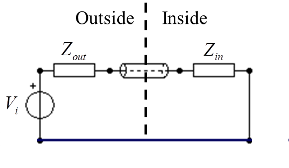
Referring to Fig. 1, we define the shielding effectiveness (SE) as the ratio of the incident power on the outside to the transmitted power on the inside of the volume shield, i.e.,

 

 

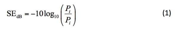
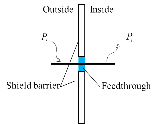
For a perfect shield the SE will be infinite and without the shield it will be 0 dB. With this as the basis we are now interested in what the SE will be when we have a shielded cable penetrating the shield. Since we here only are interested in the performance of the feedthrough itself, coloured in Fig. 1, we replace the shielded cable with a perfectly conducting rod or tube.

This is important since the SE will otherwise be a combination of the leakage through the cable shield and the leakage due to the non-perfect feedthrough.

 

For simplicity we also assume the rod to be straight and perpendicular to the shielded barrier on both sides of the shield. It is then realized that we can model the rod as two simple monopoles, one on each side of the shielded barrier. The monopole on the outside is excited by the incident field, and the monopole on the inside is, if excited, radiating on the inside. The field radiated by the monopole on the inside of the volume shield is thus the source of P_t in (1). A simple circuit equivalent model is shown in Fig. 2.

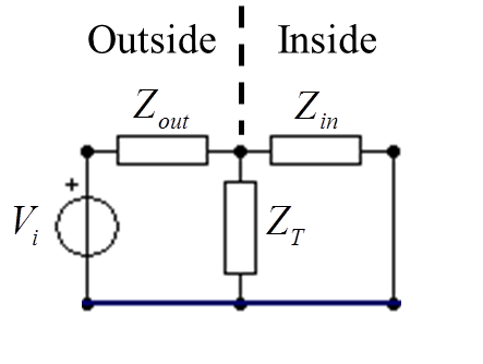
In Fig. 2 Z_out and Z_in represent the impedances of the monopoles on the outside and inside of the shielded barrier, respectively. Z_T is the total transfer impedance for the feedthrough which is composed by the contact impedance between the rod (cable shield) and the feedthrough, the impedance in the feedthrough itself and the contact impedance between the feedthrough and the shielded barrier. Finally, the voltage source V_i represents the voltage induced by the incident field.

 

From Fig. 2 we can separate out two special cases; when the feedthrough transfer impedance is zero and when it is infinite. When Z_T = 0 the monopole on the inside is short circuited and therefore not excited. In this case the SE will be infinite. In a measurement situation this case should be measured without the rod and feedthrough in place, i.e., with as good shielding as possible.

 

This will give the upper limit for SE that can be measured with the given setup. The case when Z_T = ∞ represents the case when we have no feedthrough, i.e., the rod penetrates the shield without any electrical contact with the shielded barrier. This is the worst possible case and the SE will be low, and represents the lower bound for SE that can be measured. The circuit equivalent model when Z_T = ∞ is shown in Fig. 3.

In Fig. 3 we have added a transmission line with a length equal to the thickness of the shielded barrier. If the hole in the shield is circular this will be a short coaxial line for which we easily can calculate the characteristic impedance. It should however be noted that it is only necessary to include this short transmission line for high frequencies, i.e., when the thickness of the shielded barrier starts to become comparable to the wavelength.

 

Neglecting the short transmission line, we can from Fig. 3 see that maximum power is transferred to the monopole on the inside (Z_in) when we have a conjugate impedance match, i.e., when Z_in = Z*_out. If we for a moment assume the two monopoles to have the same length, then Z_in will be equal to Z_out and we will have a conjugate impedance match only at resonances where the imaginary part of the impedance for the monopole is zero. At those frequencies the SE will have a minimum.

 

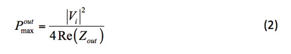
If we assume the monopoles to be lossless it is natural to define the SE in a way such that this minimum equals 0 dB. This can be assured by letting P_i in (1) be equal to the maximum power the monopole on the outside can deliver to a matched load. Thus, we in the following define SE as the ratio between the maximum power the monopole on the outside can deliver to a matched load to the power radiated by the monopole on the inside of the shielded volume.

 

For the general case when the two monopoles have different lengths, i.e., when Z_in ≠ Z_out, and referring to Fig.3 (and again neglecting the short transmission line), the method to compute SE will be as follows;

 

Compute the maximum power the monopole on the outside can deliver to a matched load.

2. Compute the power radiated by the monopole on the inside when it is excited by the monopole on the outside.

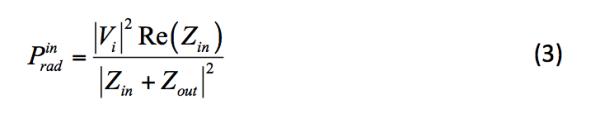
3. Compute SE as the ratio;

 

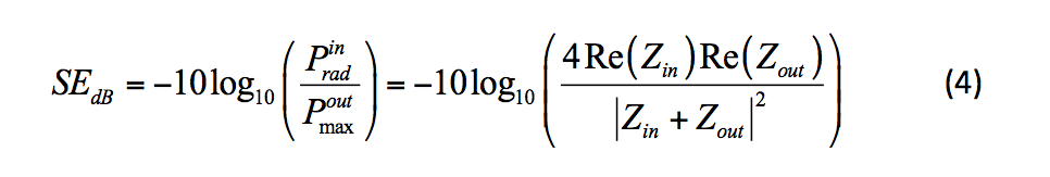
It is worth noting that the expression for SE in (4) is independent of the voltage source V_i, thus the field excitation, as it should. It should also be mentioned that the same procedure can be used for computing the SE when we have a feedthrough modelled as transfer impedance, as in Fig. 2. The expression for the power radiated by the monopole on the inside (P_in/rad) will of course be different from (3), as will the last part of (4).

 

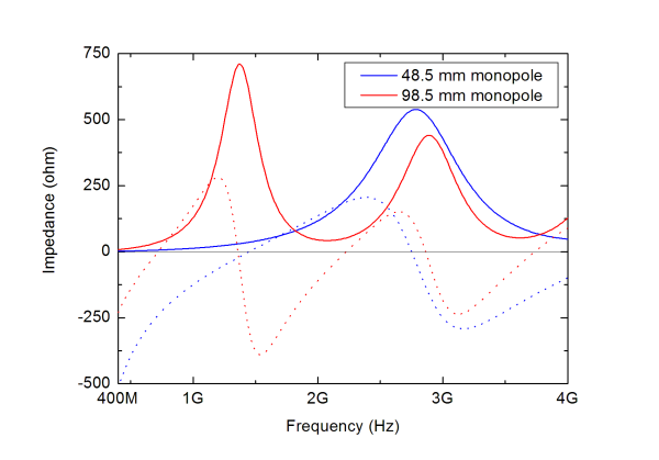
From (4) we can also readily see that if Z_in = Z_out (equally long monopoles) and the impedance is real (at resonances), SE is equal to 0 dB. For the general case we need to know the impedances for the monopoles on each side for computing the SE using the above formulas. These can easily be computed numerically using any full wave method. The examples shown in Fig. 4 were obtained using an in-house method of moments code.

 

The shielding effectiveness (SE) computed using the simple circuit approach described above, are for a few examples shown in Fig. 5-6. In order to mimic the measurement situation presented in following sections we have here included the transmission line as a 3 mm long line corresponding to the thickness of the shield used in the measurements. Given a wire radius of 0.5 mm and a radius of the circular hole in the shield of 3.75 mm, the characteristic impedance was calculated to be 121 ohm.

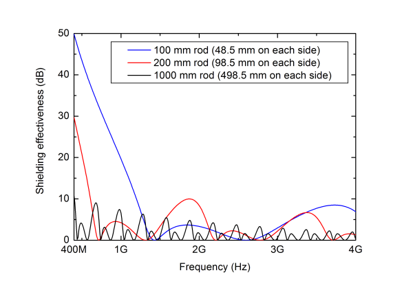
From Fig. 5 it can be noted that SE will be 0 dB at frequencies where lengths of the rods penetrating the shield correspond to resonances. It can also be seen that we need a certain length in order to be able to measure also feedthroughs with bad performance; we need e.g. a rod longer than 100 mm to be able to measure a feedthrough which have a SE of 50 dB or less at 400 MHz. From the figure it can also be concluded that in order to have as large as possible dynamic range we need a long rod, typically longer than one wavelength on each side.

In Fig. 5 it can be seen that the SE will be lower than 10 dB in the whole frequency range 0.4 to 4 GHz if the rod has a length of 1 m.

 

III. Measurement Method

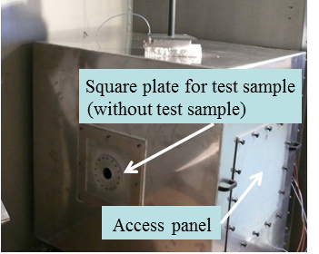
In order to validate the simple theoretical model presented in the previous section and for characterizing real cable feedthroughs we used a measurement setup with nested reverberation chambers. The method is well documented in [2] and [3] so we will not go into details here. In our setup we used a small reverberation chamber with the dimensions 0.85 by 1.2 by 1.2 m which was placed inside another chamber with dimensions 2.5 by 2.5 by 3.1 m. The test sample was mounted on a square aluminium plate with dimensions 300 by 300 mm and thickness 3 mm. This plate was mounted in one of the walls of the smaller inner chamber, see Fig. 6.

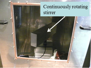
The field in the outer chamber was stirred by two metallic plate stirrers that were rotated in discrete steps. We used 8 steps for one of the stirrers while the other was rotated in 30 steps, giving a total of 240 samples. In the smaller inner chamber a single stirrer was continuously rotating with a speed of approx. 20 rpm, Fig. 7.

 

In addition to the mechanical stirring we used frequency stirring corresponding to a bandwidth of approximately 50 MHz. With the given dimensions of the chambers we were able to measure down to approximately 400 MHz.

As explained in [2] the measurement method we have used gives the SE as the ratio of two average cross sections (averaged over incidence directions and polarizations). Since this definition is not the same as our definition of SE as given by (1), we need to correct the measured results in order to be able to compare computations and measurements. In order to find the correction factor we start with the definition of the measured quantity, M,

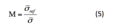
where σ_ref is the average cross section without the test sample, and σ is the average cross section with the test sample mounted. In our case the reference cross section is that of a rectangular aperture of the size 300 by 300 mm, i.e., referring to Fig. 6 without the test plate mounted. As was shown in [3] this aperture is large in terms of the wavelength for all frequencies considered here, i.e., for frequencies higher than 400 MHz. We can then use the geometrical optics approximation, from which it is found [4],

 

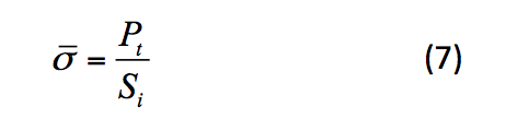
where A_ap is the physical area of the aperture, i.e., in our case 0.09 m². The cross section σ in (5) is given by the ratio of the power transmitted on the inside of the shielded volume (the small chamber in our measurement setup), P_t, to the power density on the outside (in the large chamber), S_i. Thus we have,

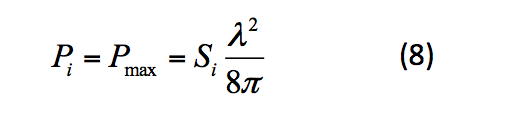
Our definition of SE is given by (1) where we, as argued for in Sect. II, define P_i to be the maximum power the monopole on the outside of the shielded volume can deliver in a matched load. This maximum power can be written as the product of the power density and an effective area. From [4] the maximum power the monopole, and in fact any lossless antenna in a well-stirred reverberation chamber, can deliver in a matched load can be written as,

 

Now putting it all together we get,

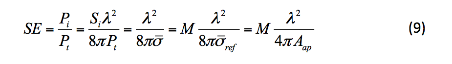
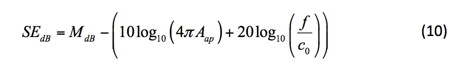
Thus, in order to compare measured results with computed, we need to multiply the measured values with the correction factor as given by (9). In Decibels we get,

IV. Results

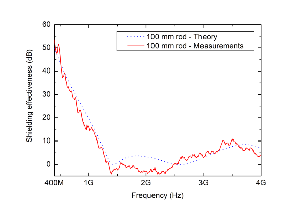
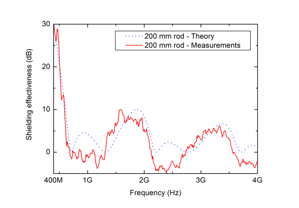
A comparison between the theory presented in Sect. II and measurements for isolated rods with different lengths are shown in Fig. 8-9. This corresponds to the case without a feedthrough as depicted in Fig. 3. As can be seen from the figures the agreement is good, typically within 5 dB or better, in the whole considered frequency range 0.4 to 4 GHz.

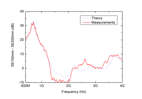
Even though the agreement between computed and measured SE is good, it is of interest to do a comparison without the influence of the correction factor given by (10). This is shown Fig. 10 where the difference between the SE for the rod with a length of 100 mm and the one with a length of 200 mm is shown. As can be seen in the figure the agreement is about the same as in Fig. 8-9.

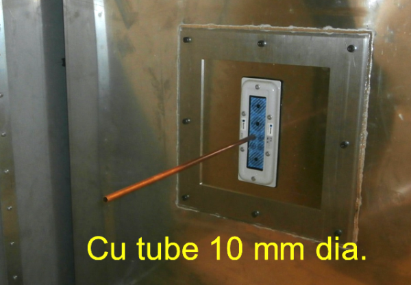
Finally, we also performed measurements on real cable feedthroughs, a few examples are presented in the following.

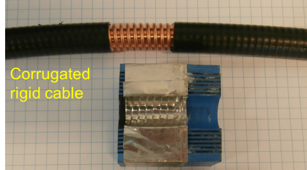
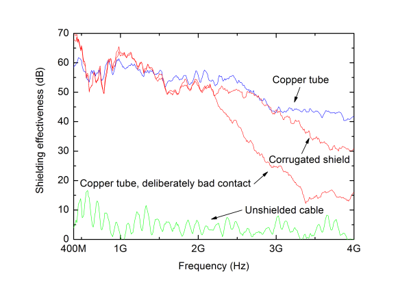
As expected, the copper tube performs very well as can be seen in Fig. 13. This curve shows in fact the maximum SE that can be measured with the instrumentation and setup that were used for the measurements. We can also see that the corrugated shielded cable also gives high SE values except at high frequencies. This could perhaps be improved by tighten the feedthrough a little bit more.

 

The effect of not tighten the feedthrough according to the manufacturer’s instructions is also shown in Fig. 13. We can see that this is especially important for high frequencies. Finally, we note that penetrating the shield with an unshielded cable is devastating; the SE will be very low.

V. Conclusions

We have presented a simple theory for how the shielding effectiveness is affected when a shield is penetrated with an isolated conductor. The theory is based on basic circuit and antenna theory and computed shielding effectiveness using the simple circuit equivalent model agrees well with measurements using nested reverberation chambers for the whole considered frequency range 0.4 to 4 GHz.

We have also presented measurement results for commercially available cable feedthroughs and shown that the proposed measurement method is viable and represents an alternative to the traditional transfer impedance method.

 

Jan Carlsson, Kristian Karlsson

SP Technical Research Institute of Sweden

 

References

1. IEC 62153-4-10, “Metallic communication cable test methods – Part 4-10: Electromagnetic compatibility (EMC) – Shielded screening attenuation method for measuring the screening effectiveness of feed-throughs and electromagnetic gaskets double coaxial method. Edition 1.0 2009-05.
2. L. Holloway, D. A. Hill, J. Ladbury, G. Koepke, and R. Garzia, “Shielding effectiveness measurements of materials using nested reverberation chambers”, IEEE Trans. Electromagn. Compat., vol. 45, no. 2, pp. 350-356, May 2003.
3. Carlsson, K. Karlsson, A. Johansson, “Validation of shielding effectiveness measurement method using nested reverberation chambers by comparison with aperture theory”, EMC Europe 2012, 11th International Symposium on EMC, Rome, Italy, 17-21 Sept., 2012.
4. A. Hill, M. T. Ma, A. R. Ondrejka, B. F. Riddle, M. L. Crawford and R. T. Johnk, “Aperture Excitation of Electrically Large, Lossy Cavities”, IEEE Trans. Electromagn. Compat., vol. 36, no. 3, pp. 169-178, Aug. 1994.